Decision by Vetocracy

Few would mistake the process of academic paper review for a fair process, but sometimes the unfairness seems particularly striking. This is most easily seen by comparison:

Paper Banditron Offset Tree Notes
Problem Scope Multiclass problems where only the loss of one choice can be probed. Strictly greater: Cost sensitive multiclass problems where only the loss of one choice can be probed. Often generalizations don’t matter. That’s not the case here, since every plausible application I’ve thought of involves loss functions substantially different from 0/1.
What’s new Analysis and Experiments Algorithm, Analysis, and Experiments As far as I know, the essence of the more general problem was first stated and analyzed with the EXP4 algorithm (page 16) (1998). It’s also the time horizon 1 simplification of the Reinforcement Learning setting for the random trajectory method (page 15) (2002). The Banditron algorithm itself is functionally identical to One-Step RL with Traces (page 122) (2003) in Bianca‘s thesis with the epsilon greedy strategy and a multiclass perceptron with update scaled by the importance weight.
Computational Time O(k) per example where k is the number of choices O(log k) per example Lower bounds on the sample complexity of learning in this setting are a factor of k worse than for supervised learning, implying that many more examples may be needed in practice. Consequently, learning algorithm speed is more important than in standard supervised learning.
Analysis Incomparable. An online regret analysis showing that if a small hinge loss predictor exists, a bounded number of mistakes occur. Also, an algorithm independent analysis of the fully realizable case. Incomparable. A learning reduction analysis showing how the regret of any base classifier bounds policy regret. Also contains a lower bound and comparable analysis of all plausible alternative reductions.
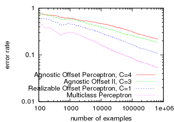
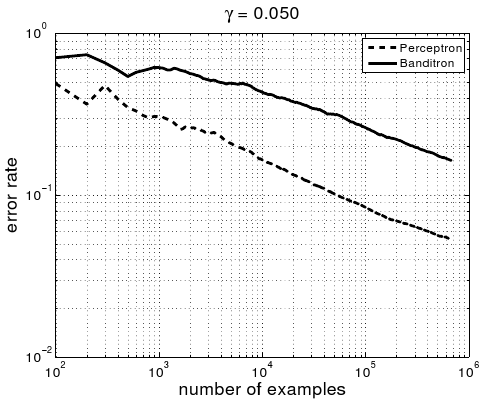
Experiments 1 dataset, comparing with no other approaches to solving the problem. 13 datasets, comparing with 2 other approaches to solve the problem.
Outcome Accepted at ICML Rejected at ICML, NIPS, UAI, and NIPS.

The reviewers of the Banditron paper made the right call. The subject is interesting, and analysis of a new learning domain is of substantial interest. Real advances in machine learning often come as new domains of application. The talk was well attended and generated substantial interest. It’s also important to remember the reviewers of the two papers probably did not overlap, so there was no explicit preference for A over B.

Why was the Offset Tree rejected? One of these rejections is easily explained as a fluke—we ran into a reviewer at UAI who believes that learning by memorization is the way to go. I, and virtually all machine learning people, disagree but some reviewers at UAI aren’t interested or expert in machine learning.

The striking thing about the other 3 rejects is that they all contain a reviewer who doesn’t read the paper. Instead, the reviewer asserts that learning reductions are bogus because for an alternative notion of learning reduction, made up by the reviewer, an obviously useless approach yields a factor of 2 regret bound. I believe this is the same reviewer each time, because the alternative theorem statement drifted over the reviews fixing bugs we pointed out in the author response.

The first time we encountered this review, we assumed the reviewer was just cranky that day—maybe we weren’t quite clear enough in explaining everything as it’s always difficult to get every detail clear in new subject matter. I have sometimes had a very strong negative impression of a paper which later turned out to be unjustified upon further consideration. Sometimes when a reviewer is cranky, they change their mind after the authors respond, or perhaps later, or perhaps never but you get a new set of reviewers the next time.

The second time the review came up, we knew there was a problem. If we are generous to the reviewer, and taking into account the fact that learning reduction analysis is a relatively new form of analysis, the fear that because an alternative notion of reduction is vacuous our notion of reduction might also be vacuous isn’t too outlandish. Fortunately, there is a way to completely address that—we added an algorithm independent lower bound to the draft (which was the only significant change in content over the submissions). This lower bound conclusively proves that our notion of learning reduction is not vacuous as is the reviewer’s notion of learning reduction.

The review came up a third time. Despite pointing out the lower bound quite explicitly, the reviewer simply ignored it. This more-or-less confirms our worst fears. Some reviewer is bidding for the paper with the intent to torpedo review it. They are uninterested in and unwiling to read the content itself.

Shouldn’t author feedback address this? Not if the reviewer ignores it.

Shouldn’t Double Blind reviewing help? Not if the paper only has one plausible source. The general problem area and method of analysis were freely discussed on hunch.net. We withheld public discussion of the algorithm itself for much of the time (except for a talk at CMU) out of respect for the review process.

Why doesn’t the area chair/program chair catch it? It took us 3 interactions to get it, so it seems unrealistic to expect someone else to get it in one interaction. In general, these people are strongly overloaded and the reviewer wasn’t kind enough to boil down the essence of the stated objection as I’ve done above. Instead, they phrase it as an example and do not clearly state the theorem they have in mind or distinguish the fact that the quantification of that theorem differs from the quantification of our theorems. More generally, my observation is that area chairs rarely override negative reviews because:

  1. It risks their reputation since defending a criticized work requires the kind of confidence that can only be inspired by a thorough personal review they don’t have time for.
  2. They may offend the reviewer they invited to review and personally know.
  3. They figure that the average review is similar to the average perception/popularity by the community anyways.
  4. Even if they don’t agree with the reviewer, it’s hard to fully discount the review in their consideration.

I’ve seen these effects create substantial mental gymnastics elsewhere.

Maybe you just ran into a cranky reviewer 3 times randomly Maybe so. However, the odds seem low enough and the 1/2 year cost of getting another sample high enough, that going with the working hypothesis seems indicated.

Maybe the writing needs improving. Often that’s a reasonable answer for a rejection, but in this case I believe not. We’ve run the paper by several people, who did not have substantial difficulties understanding it. They even understand the draft well enough to make a suggestion or two. More generally, no paper is harder to read than the one you picked because you want to reject it.

What happens next? With respect to the Offset Tree, I’m hopeful that we eventually find reviewers who appreciate an exponentially faster algorithm, good empirical results, or the very tight and elegant analysis, or even all three. For the record, I consider the Offset Tree a great paper. It remains a substantial advance on the state of the art, even 2 years later, and as far as I know the Offset Tree (or the Realizable Offset Tree) consistently beat all reasonable contenders both in prediction and computational performance. This is rare and precious, as many papers tradeoff one for the other. It yields a practical algorithm applicable to real problems. It substantially addresses the RL to classification reduction problem. It also has the first nonconstant algorithm independent lower bound for learning reductions.

With respect to the reviewer, I expect remarkably little. The system is designed to protect reviewers, so they have virtually no responsibility for their decisions. This reviewer has a demonstrated capability to sabotage the review process at ICML and NIPS and a demonstrated willingness to continue doing so indefinitely. The process of bidding for papers and making up reasons to reject them seems tedious, but there is no fundamental reason why they can’t continue doing so for several decades if they remain active in academia.

This experience has substantially altered my understanding and appreciation of the review process at conferences. The bidding mechanism commonly used, coupled with responsibility-free reviewing is an invitation to abuse. A clever abusive reviewer can sabotage perhaps 5 papers per conference (out of 8 reviewed), while maintaining a typical average score. While I don’t believe most people choose papers with intent to sabotage, the capability is there and used by at least one person and possibly others. If, for example, 5% of reviewers are willing to abuse the process this way and there are 100 reviewers, every paper must survive 5 vetoes. If there are 200 reviewers, every paper must survive 10 vetoes. And if there are 400 reviewers, every paper must survive 20 vetoes. This makes publishing any paper that offends someone difficult. The surviving papers are typically inoffensive or part of a fad strong enough that vetoes are held back. Neither category is representative of high quality decision making. These observations suggest that the conference with the most reviewers tend strongly toward faddy and inoffensive papers, both of which often lack impact in the long term. Perhaps this partly explains why NIPS is so weak when people start citation counting. Conversely, this would suggest that smaller conferences and workshops have a natural advantage. Similarly, the reviewing style in theory conferences seems better—the set of bidders for any paper is substantially smaller, implying papers must survive fewer vetos.

This decision making process can be modeled as a group of n decision makers, each of which has the opportunity to veto any action. When n is relatively small, this decision making process might work ok, depending on the decision makers, but as n grows larger, it’s difficult to imagine a worse decision making process. The closest representatives outside of academia I know are deeply bureacratic governments and other large organizations where many people must sign off on something before it takes place. These vetocracies are universally frustrating to interact with. A reasonable conjecture is that any decision making process with a large veto number has poor characteristics.

A basic question is: Is a vetocracy inevitable for large organizations? I believe the answer is no. The basic observation is that the value of n can be logarithmic in the number of participants in an organization rather than linear, as per reviewing under a bidding process. An essential force driving vetocracy creation is a desire to offload responsibility for decisions, so there is no clear decision maker. A large organization not deciding by vetocracy must have a very different structure, with clearly dilineated responsibility.

NIPS provides an almost perfect natural experiment in it’s workshop organization, which involves the very same community of people and subject matter, yet works in a very different manner. There are one or two workshop chairs who are responsible for selecting amongst workshop proposals, after which the content of the workshop is entirely up to the workshop organizers. If a workshop is rejected, it’s clear who is at fault, and if a workshop presentation is rejected, it is often clear by who. Some workshop chairs use a small set of reviewers, but even then the effective veto number remains small. Similarly, if a workshop ends up a flop, it’s relatively easy to see who to blame—either the workshop chair for not predicting it, or the organizers for failing to organize. I can’t think of a single time when I attended both the workshops and the conference that the workshops were less interesting than the conference. My understanding is that this observation is common. Given this discussion, it will be particularly interesting to see how the review process Michael and Leon setup for ICML this year pans out, as it is a system with notably more responsibility assignment than in previous years.

Journals end up looking relatively good with respect to vetocracy avoidance. The ones I’m familiar with have a chief editor who bears responsibility for routing papers to an action editor, who bears responsibility for choosing good reviewers. Every agent except the reviewers is often known by the authors, and the reviewers don’t act as additional vetoers in nearly as strong a manner as reviewers with the opportunity to bid.

This experience has also altered my view of blogging and research. On one hand, I’m very enthusiastic about research in general, and my research in particular, where we are regularly cracking conventionally impossible problems. On the other hand, it seems that some small number of people viewing a discussion silently decide they don’t like it, and veto it given the opportunity. It only takes one to turn strong paper into a years-long odyssey, so public discussion of research directions and topics in a vetocracy is akin to voluntarily wearing a “kick me” sign. While this a problem for me, I expect it to be even worse for the members of a vetocracy in the long term.

It’s hard to imagine any research community surviving without a serious online presence. When a prospective new researcher looks around at existing research, if they don’t find serious online discussion, they’ll assume it doesn’t exist under the “not on the internet so it doesn’t exist” principle. This will starve a field of new people. More generally, there is an opportunity to get feedback about research directions and problems much more rapidly than is otherwise possible, allowing us to avoid research on dead end topics which are pervasive. At some point, it may even seem that people not willing to discuss their research simply avoid doing so because it is critically lacking in one way or another. Since a vetocracy creates a substantial disincentive to discuss research directions online, we can expect that communities sticking with decision by vetocracy to be at a substantial disadvantage.

Optimal Proxy Loss for Classification

Many people in machine learning take advantage of the notion of a proxy loss: A loss function which is much easier to optimize computationally than the loss function imposed by the world. A canonical example is when we want to learn a weight vector w and predict according to a dot product fw(x)= sumi wixi
where optimizing squared loss (y-fw(x))2 over many samples is much more tractable than optimizing 0-1 loss I(y = Threshold(fw(x) – 0.5)).

While the computational advantages of optimizing a proxy loss are substantial, we are curious: which proxy loss is best? The answer of course depends on what the real loss imposed by the world is. For 0-1 loss classification, there are adherents to many choices:

  1. Log loss. If we confine the prediction to [0,1], we can treat it as a predicted probability that the label is 1, and measure loss according to log 1/p'(y|x) where p'(y|x) is the predicted probability of the observed label. A standard method for confining the prediction to [0,1] is logistic regression which exponentiates the dot product and normalizes.
  2. Squared loss. The squared loss approach (discussed above) is also quite common. It shares the same “proper scoring rule” semantics as log loss: the optimal representation-independent predictor is the conditional probability of the label y given the features x.
  3. Hinge loss. For hinge loss, you optimize max(0, 1- 4 (y – 0.5) (fw(x) – 0.5) ). The form of hinge loss is slightly unfamiliar, because the label is {0,1} rather than {-1,1}. The optimal prediction for hinge loss is not the probability of y given x but rather some value which is at least 1 if the most likely label is 1 and 0 or smaller if the most likely label is 0. Hinge loss was popularized with support vector machines. Hinge loss is not a proper scoring rule for mean, but since it does get the sign right, using it for classification is reasonable.

Many people have made qualitative arguments about why one loss is better than another. For example see Yaroslav’s old post for an argument about the comparison of log loss and hinge loss and why hinge loss might be better. In the following, I make an elementary quantitative argument.

Log loss is qualitatively dissimilar from the other two, because it is unbounded on the range of interest. Restated, there is no reason other than representational convenience that fw(x) needs to take a value outside of the interval [0,1] for squared loss or hinge loss. In fact, we can freely reduce these losses by considering instead the function fw‘(x) = max(0,min(1,fw(x))). The implication is that optimization of log loss can be unstable in ways that optimization of these other losses is not. This can be stated precisely by noting that sample complexity bounds (simple ones here) for 0-1 loss hold for fw‘(x) under squared or hinge loss, but the same theorem statement does not hold for log loss without additional assumptions. Since stability and convergence are of substantial interest in machine learning, this suggests not using log loss.

For further analysis, we must first define some function converting fw(x) into label predictions. The only reasonable approach is to threshold at 0.5. For log loss and squared loss, any other threshold is inconsistent. Since the optimal predictor for hinge loss always takes value 0 or 1, there is some freedom in how we convert, but a reasonable approach is to also threshold at 0.5.

Now, we want to analyze the stability of predictions. In other words, if an adversary picks the true conditional probability distribution p(y|x) and the prediction fw‘(x), how does the proxy loss of fw‘(x) bound the 0-1 loss? Since we imagine that the conditional distribution is noisy, it’s important to actually consider a regret: how well we do minus the loss of the best possible predictor.

For each of these losses, an optimal strategy of the adversary is to have p(y|x) take value 0.5 – eps and fw‘(x) = 0.5. The 0-1 regret induced is simply 2 eps, since the best possible predictor has error rate 0.5 – eps while the actual predictor has error rate 0.5 + eps. For hinge loss, the regret is eps and for squared loss the regret is eps2. Doing some algebra, this implies that 2 hinge_regret bounds 0-1 regret while 2 squared_regret0.5 bounds 0-1 regret. Since we are only interested in regrets less than 1, the square root is undesirable, and hinge loss is preferred, because a stronger convergence of squared loss is needed to achieve the same guarantee on 0-1 loss.

Can we improve on hinge loss? I don’t know any proxy loss which is quantitatively better, but generalizations exist. The regret of hinge loss is the same as for absolute value loss |y-fw‘(x)| since they are identical for 0,1 labels. One advantage of absolute value loss is that it has a known and sometimes useful semantics for values between 0 and 1: the optimal prediction is the median. This makes the work on quantile regression (Two Three) seem particularly relevant for machine learning.

Observations on Linearity for Reductions to Regression

Dean Foster and Daniel Hsu had a couple observations about reductions to regression that I wanted to share. This will make the most sense for people familiar with error correcting output codes (see the tutorial, page 11).

Many people are comfortable using linear regression in a one-against-all style, where you try to predict the probability of choice i vs other classes, yet they are not comfortable with more complex error correcting codes because they fear that they create harder problems. This fear turns out to be mathematically incoherent under a linear representation: comfort in the linear case should imply comfort with more complex codes.

In particular, If there exists a set of weight vectors wi such that P(i|x)= <wi,x>, then for any invertible error correcting output code C, there exists weight vectors wc which decode to perfectly predict the probability of each class. The proof is simple and constructive: the weight vector wc can be constructed according to the linear superposition of wi implied by the code, and invertibility implies that a correct encoding implies a correct decoding.

This observation extends to all-pairs like codes which compare subsets of choices to subsets of choices using “don’t cares”.

Using this observation, Daniel created a very short proof of the PECOC regret transform theorem (here, and Daniel’s updated version).

One further observation is that under ridge regression (a special case of linear regression), for any code, there exists a setting of parameters such that you might as well use one-against-all instead, because you get the same answer numerically. The implication is that the advantages of codes more complex than one-against-all is confined to other prediction methods.

Compositional Machine Learning Algorithm Design

There were two papers at ICML presenting learning algorithms for a contextual bandit-style setting, where the loss for all labels is not known, but the loss for one label is known. (The first might require a exploration scavenging viewpoint to understand if the experimental assignment was nonrandom.) I strongly approve of these papers and further work in this setting and its variants, because I expect it to become more important than supervised learning. As a quick review, we are thinking about situations where repeatedly:

  1. The world reveals feature values (aka context information).
  2. A policy chooses an action.
  3. The world provides a reward.

Sometimes this is done in an online fashion where the policy can change based on immediate feedback and sometimes it’s done in a batch setting where many samples are collected before the policy can change. If you haven’t spent time thinking about the setting, you might want to because there are many natural applications.

I’m going to pick on the Banditron paper (second one), which attacks the special case of the contextual bandit setting where exactly one of the rewards is 1 and all other actions result in reward 0, and show that (a) similar performance is achievable via a simple combination of existing modular technologies and (b) superior performance is achievable by optimizing some existing modular technologies for the realizable case. This algorithm is the hardest of the two to compete with, because it explicitly deals with the explore/exploit tradeoff. Note that I’m definitely not trying to minimize the paper—there is analysis in that paper which remains interesting to me and isn’t covered by what follows. I am happy that it was published. The point of this post is showing that a modular approach to building learning algorithms is a strong contender when we encounter new learning problems.

Given the problem statement, my approach to solving the problem would be to compose some modular technologies I know.

  1. Perceptron learning algorithm We chose a Binary Perceptron as a classification algorithm. This choice is intrinsically motivated by the great computational performance of a Perceptron. It’s also the closest binary supervised learning algorithm to the Banditron, which eliminates a source of variation in comparison. We could have easily chosen a different base learning algorithm, and in many applications this is highly desirable.
  2. Offset Tree Reduction The offset tree is a newer machine learning reduction from the contextual bandit setting to the standard supervised learning setting. It more robustly transforms a supervised learner’s performance into good policy performance than any other reduction. The offset tree also has good computational properties, since it produces at most log2 k binary examples per train or test event, where k is the number of actions. In some sense it’s unfair to include the offset tree because it hasn’t yet been formally published. In another sense, that’s what this post is about.
  3. Epoch-Greedy exploration. The Epoch-greedy approach shows how to handle the explore/exploit tradeoff for learning in a contextual bandit setting as a function of a sample complexity bound. For common sample complexity bounds, we get an O(T2/3) online regret where T is the total number of timesteps.
  4. Occam’s Razor Bound The Occam’s Razor bound limits the regret of an empirical error minimizing perceptron as function of the number of examples. The bound (and it’s many cousins) are often loose, so the only thing we’ll really use is the denominator which says that regret scales as 1/sqrt(number of training examples) in the worst case. Applying Epoch-Greedy to the Occam’s Razor bound gives you an exploration probability of about C/t1/3 where t is the round number.

Each component above has been analyzed in isolation and is at least a reasonable approach (some are the best possible). Each of these components is also composable. Fitting these pieces together, we get an online learning algorithm (agnostic offset-tree perceptron) that chooses to explore uniformly at random amongst the actions with probability about 1/t1/3. How well does it perform? On the 4 class reuters based dataset used in the Banditron paper, we get the following accumulated average error rates with some code.:

The right plot is from the Banditron paper. The Perceptron line in both plots is for an algorithm which learns knowing the full loss function of each example, so it represents an ideal we don’t expect to achieve here. There are three results in the left plot:

  1. The blue line is a version of the component set where the Occam’s Razor bound and the Offset Tree reduction have been optimized for the realizable case. This was the first thing we tested (and it’s the result I mentioned at Shai‘s ICML talk). It turns out this approach works substantially better than the Banditron, achieving an error rate about halfway between the Banditron and the Multiclass Perceptron. The two components that we tweaked are:
    1. Realizable case Bound It’s well known that in the realizable case the regret of a chosen classifier should scale as 1/t rather than 1/t0.5. Plugging this into epoch-greedy, we get that the probability of exploration should be about 1/t0.5.
    2. Realizable case Offset Tree A basic observation is that in the realizable setting, every observation should create an example to tune the learning algorithm. In the context of the perceptron, this implies every error creates an example. The offset tree reduction can be altered to take this into account by eliminating the importance weight from all updates, and updating even for exploitation examples which are not drawn uniform randomly.
  2. The red line is what you get with exactly the component set stated above. We were curious about the degree to which a general purpose algorithm can perform well on this application as the realizable case algorithm is definitely broken when the problem is inherently noisy. The performance is somewhat worse than Banditron. I believe this is because it explores only about 1% of the time while the Banditron plot comes from exploring about 5% of the time.
  3. The green line is from a component set where epoch greedy and the offset tree have been tweaked to keep track of and use the distribution over actions at every timestep. This tweaks allows the amount of exploration as measured by the sum of importance weights of training examples to almost double. As we see, this approach improves performance, almost as if we doubled the number of examples, giving it similar performance to the Banditron. The tweaks used for the component set are:
    1. Stochastic Epoch-Greedy Instead of deterministically exploring every 1/(bound_gap) times, choose to explore with probability 1/(bound_gap), and pass this probability to the offset tree reduction.
    2. Nonuniform Offset Tree Tweak the Offset Tree in the obvious way to take into account nonuniform exploration. In particular, 1/2 is replaced with K/p(a) where p(a) is the probability of the action taken conditioned on one of two actions being taken. We set K so that this value is 1 when a nonexploit action is taken, which implies the importance weight is p(a)/(2-p(a)) when the exploit action is taken.
    3. Importance Weighted Perceptron We dealt with importance weights generated by the offset tree reduction by scaling any update by the importance weight.

People may be dissatisfied with the component assembly approach to learning algorithm design, because all of the pieces are not analyzed together. For example, the Banditron paper essentially proves that certain conditions are sufficient for the Banditron algorithm to perform well. This is a more complete guarantee than “all the pieces we stuck together are known to work well when analyzed in isolation”, but this style of guarantee has limitations which are both obvious and often overlooked. These guarantees do not show necessity of these conditions, and hence characterize only a subset of settings where the Banditron works. Unless you are lucky enough to know that your application satisfies the sufficient conditions, you’ll basically have to try the Banditron and see if it works for any particular application. Another drawback is that the complexity of analyzing all the different pieces simultaneously means that it’s difficult to use the best elements together. This last point is what leaves me dissatisfied with the complete analysis approach—it produces algorithms which are simple to analyze rather than optimized for performance.

If you are thinking “I have a better algorithm for solving one problem”, then you’ve missed the point of this post. The point of this post is that compositional design is good for solving many learning problems. This post is about one example of that approach in action. We start by assembling a set of components which we know work well from individual component analysis. Then, we try to optimize the performance of the assembly by swapping components or improving individual components to address known properties of the problem or observed deficiencies. In this particular case, we end up with a better performing algorithm and better components (such as stochastic epoch greedy) which are directly reusable in other settings. The essence of this approach is understanding that there is a real vocabulary of interchangeable components and actively using it in designing learning algorithms.

I would like to thank Alina who helped substantially with this post. I would also like to thank Shai for providing data and helping setup a clean comparison and Sham for helpful discussion.

Computational Consequences of Classification

In the regression vs classification debate, I’m adding a new “pro” to classification. It seems there are computational shortcuts available for classification which simply aren’t available for regression. This arises in several situations.

  1. In active learning it is sometimes possible to find an e error classifier with just log(e) labeled samples. Only much more modest improvements appear to be achievable for squared loss regression. The essential reason is that the loss function on many examples is flat with respect to large variations in the parameter spaces of a learned classifier, which implies that many of these classifiers do not need to be considered. In contrast, for squared loss regression, most substantial variations in the parameter space influence the loss at most points.
  2. In budgeted learning, where there is either a computational time constraint or a feature cost constraint, a classifier can sometimes be learned to very high accuracy under the constraints while a squared loss regressor could not. For example, if there is one feature which determines whether a binary label has probability less than or greater than 0.5, a great classifier exists using just one feature. Because squared loss is sensitive to the exact probability, many more features may be required to learn well with respect to squared loss.