There were two papers at ICML presenting learning algorithms for a contextual bandit-style setting, where the loss for all labels is not known, but the loss for one label is known. (The first might require a exploration scavenging viewpoint to understand if the experimental assignment was nonrandom.) I strongly approve of these papers and further work in this setting and its variants, because I expect it to become more important than supervised learning. As a quick review, we are thinking about situations where repeatedly:
- The world reveals feature values (aka context information).
- A policy chooses an action.
- The world provides a reward.
Sometimes this is done in an online fashion where the policy can change based on immediate feedback and sometimes it’s done in a batch setting where many samples are collected before the policy can change. If you haven’t spent time thinking about the setting, you might want to because there are many natural applications.
I’m going to pick on the Banditron paper (second one), which attacks the special case of the contextual bandit setting where exactly one of the rewards is 1 and all other actions result in reward 0, and show that (a) similar performance is achievable via a simple combination of existing modular technologies and (b) superior performance is achievable by optimizing some existing modular technologies for the realizable case. This algorithm is the hardest of the two to compete with, because it explicitly deals with the explore/exploit tradeoff. Note that I’m definitely not trying to minimize the paper—there is analysis in that paper which remains interesting to me and isn’t covered by what follows. I am happy that it was published. The point of this post is showing that a modular approach to building learning algorithms is a strong contender when we encounter new learning problems.
Given the problem statement, my approach to solving the problem would be to compose some modular technologies I know.
- Perceptron learning algorithm We chose a Binary Perceptron as a classification algorithm. This choice is intrinsically motivated by the great computational performance of a Perceptron. It’s also the closest binary supervised learning algorithm to the Banditron, which eliminates a source of variation in comparison. We could have easily chosen a different base learning algorithm, and in many applications this is highly desirable.
- Offset Tree Reduction The offset tree is a newer machine learning reduction from the contextual bandit setting to the standard supervised learning setting. It more robustly transforms a supervised learner’s performance into good policy performance than any other reduction. The offset tree also has good computational properties, since it produces at most log2 k binary examples per train or test event, where k is the number of actions. In some sense it’s unfair to include the offset tree because it hasn’t yet been formally published. In another sense, that’s what this post is about.
- Epoch-Greedy exploration. The Epoch-greedy approach shows how to handle the explore/exploit tradeoff for learning in a contextual bandit setting as a function of a sample complexity bound. For common sample complexity bounds, we get an O(T2/3) online regret where T is the total number of timesteps.
- Occam’s Razor Bound The Occam’s Razor bound limits the regret of an empirical error minimizing perceptron as function of the number of examples. The bound (and it’s many cousins) are often loose, so the only thing we’ll really use is the denominator which says that regret scales as 1/sqrt(number of training examples) in the worst case. Applying Epoch-Greedy to the Occam’s Razor bound gives you an exploration probability of about C/t1/3 where t is the round number.
Each component above has been analyzed in isolation and is at least a reasonable approach (some are the best possible). Each of these components is also composable. Fitting these pieces together, we get an online learning algorithm (agnostic offset-tree perceptron) that chooses to explore uniformly at random amongst the actions with probability about 1/t1/3. How well does it perform? On the 4 class reuters based dataset used in the Banditron paper, we get the following accumulated average error rates with some code.:
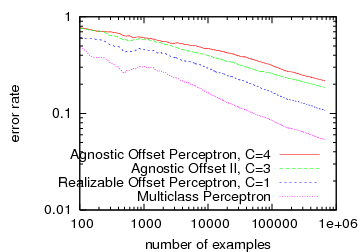
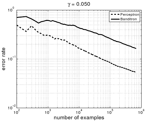
The right plot is from the Banditron paper. The Perceptron line in both plots is for an algorithm which learns knowing the full loss function of each example, so it represents an ideal we don’t expect to achieve here. There are three results in the left plot:
- The blue line is a version of the component set where the Occam’s Razor bound and the Offset Tree reduction have been optimized for the realizable case. This was the first thing we tested (and it’s the result I mentioned at Shai‘s ICML talk). It turns out this approach works substantially better than the Banditron, achieving an error rate about halfway between the Banditron and the Multiclass Perceptron. The two components that we tweaked are:
- Realizable case Bound It’s well known that in the realizable case the regret of a chosen classifier should scale as 1/t rather than 1/t0.5. Plugging this into epoch-greedy, we get that the probability of exploration should be about 1/t0.5.
- Realizable case Offset Tree A basic observation is that in the realizable setting, every observation should create an example to tune the learning algorithm. In the context of the perceptron, this implies every error creates an example. The offset tree reduction can be altered to take this into account by eliminating the importance weight from all updates, and updating even for exploitation examples which are not drawn uniform randomly.
- The red line is what you get with exactly the component set stated above. We were curious about the degree to which a general purpose algorithm can perform well on this application as the realizable case algorithm is definitely broken when the problem is inherently noisy. The performance is somewhat worse than Banditron. I believe this is because it explores only about 1% of the time while the Banditron plot comes from exploring about 5% of the time.
- The green line is from a component set where epoch greedy and the offset tree have been tweaked to keep track of and use the distribution over actions at every timestep. This tweaks allows the amount of exploration as measured by the sum of importance weights of training examples to almost double. As we see, this approach improves performance, almost as if we doubled the number of examples, giving it similar performance to the Banditron. The tweaks used for the component set are:
- Stochastic Epoch-Greedy Instead of deterministically exploring every 1/(bound_gap) times, choose to explore with probability 1/(bound_gap), and pass this probability to the offset tree reduction.
- Nonuniform Offset Tree Tweak the Offset Tree in the obvious way to take into account nonuniform exploration. In particular, 1/2 is replaced with K/p(a) where p(a) is the probability of the action taken conditioned on one of two actions being taken. We set K so that this value is 1 when a nonexploit action is taken, which implies the importance weight is p(a)/(2-p(a)) when the exploit action is taken.
- Importance Weighted Perceptron We dealt with importance weights generated by the offset tree reduction by scaling any update by the importance weight.
People may be dissatisfied with the component assembly approach to learning algorithm design, because all of the pieces are not analyzed together. For example, the Banditron paper essentially proves that certain conditions are sufficient for the Banditron algorithm to perform well. This is a more complete guarantee than “all the pieces we stuck together are known to work well when analyzed in isolation”, but this style of guarantee has limitations which are both obvious and often overlooked. These guarantees do not show necessity of these conditions, and hence characterize only a subset of settings where the Banditron works. Unless you are lucky enough to know that your application satisfies the sufficient conditions, you’ll basically have to try the Banditron and see if it works for any particular application. Another drawback is that the complexity of analyzing all the different pieces simultaneously means that it’s difficult to use the best elements together. This last point is what leaves me dissatisfied with the complete analysis approach—it produces algorithms which are simple to analyze rather than optimized for performance.
If you are thinking “I have a better algorithm for solving one problem”, then you’ve missed the point of this post. The point of this post is that compositional design is good for solving many learning problems. This post is about one example of that approach in action. We start by assembling a set of components which we know work well from individual component analysis. Then, we try to optimize the performance of the assembly by swapping components or improving individual components to address known properties of the problem or observed deficiencies. In this particular case, we end up with a better performing algorithm and better components (such as stochastic epoch greedy) which are directly reusable in other settings. The essence of this approach is understanding that there is a real vocabulary of interchangeable components and actively using it in designing learning algorithms.
I would like to thank Alina who helped substantially with this post. I would also like to thank Shai for providing data and helping setup a clean comparison and Sham for helpful discussion.