Explicit Randomization in Learning algorithms

There are a number of learning algorithms which explicitly incorporate randomness into their execution. This includes at amongst others:

  1. Neural Networks. Neural networks use randomization to assign initial weights.
  2. Boltzmann Machines/Deep Belief Networks. Boltzmann machines are something like a stochastic version of multinode logistic regression. The use of randomness is more essential in Boltzmann machines, because the predicted value at test time also uses randomness.
  3. Bagging. Bagging is a process where a learning algorithm is run several different times on several different datasets, creating a final predictor which makes a majority vote.
  4. Policy descent. Several algorithms in reinforcement learning such as Conservative Policy Iteration use random bits to create stochastic policies.
  5. Experts algorithms. Randomized weighted majority use random bits as a part of the prediction process to achieve better theoretical guarantees.

A basic question is: “Should there be explicit randomization in learning algorithms?” It seems perverse to feed extra random bits into your prediction process since they don’t contain any information about the problem itself. Can we avoid using random numbers? This question is not just philosophy—we might hope that deterministic version of learning algorithms are both more accurate and faster.

There seem to be several distinct uses for randomization.

  1. Symmetry breaking. In the case of a neural network, if every weight started as 0, the gradient of the loss with respect to every weight would be the same, implying that after updating, all weights remain the same. Using random numbers to initialize weights breaks this symmetry. It is easy to believe that there are good deterministic methods for symmetry breaking.
  2. Overfit avoidance. A basic observation is that deterministic learning algorithms tend to overfit. Bagging avoids this by randomizing the input of these learning algorithms in the hope that directions of overfit for individual predictions cancel out. Similarly, using random bits internally as in a deep belief network avoids overfitting by forcing the algorithm to learn a robust-to-noise set of internal weights, which are then robust-to-overfit. Large margin learning algorithms and maximum entropy learning algorithms can be understood as deterministic operations attempting to achieve the same goal. A significant gap remains between randomized and deterministic learning algorithms: the deterministic versions just deal with linear predictions while the randomized techniques seem to yield improvements in general.
  3. Continuizing. In reinforcement learning, it’s hard to optimize a policy over multiple timesteps because the optimal decision at timestep 2 is dependent on the decision at timestep 1 and vice versa. Randomized interpolation of policies offers a method to remove this cyclic dependency. PSDP can be understood as a derandomization of CPI which trades off increased computation (learning a new predictor for each timestep individually). Whether or not we can avoid a tradeoff in general is unclear.
  4. Adversary defeating. Some algorithms, such as randomized weighted majority are designed to work against adversaries who know your algorithm, except for random bits. The randomization here is provably essential, but the setting is often far more adversarial than the real world.

The current state-of-the-art is that random bits provide performance (computational and predictive) which we don’t know (or at least can’t prove we know) how to achieve without randomization. Can randomization be removed or is it essential to good learning algorithms?
Online convex optimization at COLT

At ICML 2003, Marty Zinkevich proposed the online convex optimization setting and showed that a particular gradient descent algorithm has regret O(T0.5) with respect to the best predictor where T is the number of rounds. This seems to be a nice model for online learning, and there has been some significant follow-up work.

At COLT 2006 Elad Hazan, Adam Kalai, Satyen Kale, and Amit Agarwal presented a modification which takes a Newton step guaranteeing O(log T) regret when the first and second derivatives are bounded. Then they applied these algorithms to portfolio management at ICML 2006 (with Robert Schapire) yielding some very fun graphs.

Explorations of Exploration

Exploration is one of the big unsolved problems in machine learning. This isn’t for lack of trying—there are many models of exploration which have been analyzed in many different ways by many different groups of people. At some point, it is worthwhile to sit back and see what has been done across these many models.

  • Reinforcement Learning (1). Reinforcement learning has traditionally focused on Markov Decision Processes where the next state s’ is given by a conditional distribution P(s’|s,a) given the current state s and action a. The typical result here is that certain specific algorithms controlling an agent can behave within e of optimal for horizon T except for poly(1/e,T,S,A) “wasted” experiences (with high probability). This started with E3 by Satinder Singh and Michael Kearns. Sham Kakade’s thesis has significant discussion. Extensions have typically been of the form “under extra assumptions, we can prove more”, for example Factored-E3 and Metric-E3. (It turns out that the number of wasted samples can be less than the number of bits required to describe an MDP.) A weakness of all these results is that they rely upon (a) assumptions which are often false for real applications, (b) state spaces are too large, and (c) make a gurantee that is rather weak. Good performance is only guaranteed after suffering the possibly catastrophic consequences of exploration.
  • Reinforcement Learning (2). Several recent papers have been attempting to analyze reinforcement learning via reduction. To date, all results are either nonconstructive or involve the use of various hints (oracle access to an optimal policy, the distribution over states of an optimal policy etc…) which short-circuit the need to explore. Obviously, these hints are not always available for real-world problems.
  • Reinforcement Learning (3). Much of the rest of reinforcement learning has something to do with exploration, but it’s difficult to summarize succinctly.
  • Online Learning. The n-armed bandit setting can be thought of as an MDP with one state and many actions. In some variants, there is even an adversary who chooses the payoffs of the arms in a non-stochastic manner. The typical result here says that you can compete well with the best constant action after some wasted actions. The exact number of wasted actions varies with the precise setting, but it is typically linear in the number of actions. This work can be traced back to (at least) Gittins indices which (unfortunately) don’t seem to have a good description available on the internet.
  • Active Learning(1) The common current use of this term has to do with “selective sampling”=choosing unlabeled samples to label so as to minimize the number of labels required to learn a good predictor (typically a classifier). A typical result has the form: Given that your classifier comes from restricted class C and the labeled data distribution obeys some constraint, the number of adaptively labeled samples required O(log (1/e)) where e is the error rate. (It turns out that the even noisy distributions are allowed.) The constraints on distributions and hypothesis spaces required to achieve these speedups are often severe.
  • Active Learning(2) Membership query learning is another example. The distinguishing difference with respect to selective sampling is that the a labeled can be requested for any unlabeled point (not just those drawn according to some natural distribution). Several relatively strong results hold for membership query learning, but there is a significant drawback: it seems that the ability to query for a label on an arbitrary point is not very natural. For example, imagine query whether a text document is about sports or politics when the text is generated at random.
  • Active Learning(3) Experimental design (which is mostly based in statistics), is often about finding the extrema of some function rather than generalization. Often, the data generating distribution is assumed to come from some specific parametric family. Unfortunately, my knowledge is sketchy here.

The striking thing about all of these models is that they fail to apply to typical real world problems. This failure is either by design (making assumptions which are simply rarely met), by failure to prove interesting results, or both.

And yet, many of the pieces are here. Active learning deals with generalization, online learning can deal with adversarial situations, and reinforcement learning deals with the situation where your choices influence what you can later learn. At a high level, there is much room for research here by design of a new model of exploration, new theoretical statements, or both.

I’ve been told “exploration is too hard”, and that’s a good warning to bear in mind, but I’m still hopeful for progress.

Online learning or online preservation of learning?

In the online learning with experts setting, you observe a set of predictions, make a decision, and then observe the truth. This process repeats indefinitely. In this setting, it is possible to prove theorems of the sort:

master algorithm error count < = k* best predictor error count + c*log(number of predictors)

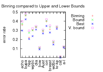
Is this a statement about learning or about preservation of learning? We did some experiments to analyze the new Binning algorithm which works in this setting. For several UCI datasets, we reprocessed them so that features could be used as predictors and then applied several master algorithms. The first graph confirms that Binning is indeed a better algorithm according to the tightness of the upper bound.


Here, “Best” is the performance of the best expert. “V. Bound” is the bound for Vovk‘s algorithm (the previous best). “Bound” is the bound for the Binning algorithm. “Binning” is the performance of the Binning algorithm. The Binning algorithm clearly has a tighter bound, and the performance bound is clearly a sharp constraint on the algorithm performance.

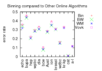
Instead of examining bounds, we can simply look at performance.


“Bin” is the performance of Binning (identical to the previous graph). BW is Binomial weighting, which is (roughly) the deterministic version of Binning. WM is Weighted Majority. Both BW and WM are deterministic algorithms which implies their performance bounds are perhaps a factor of 2 worse than Binning or Vovk’s algorithm.

In contrast, the actual performance (rather than performance bound) of the deterministic algorithms is sometimes even better than the best expert (negative regret?!). A consistent negative correlation between “online bound tightness” and “learning performance” is observed.

The question is “What’s happening here?”

  1. One reply is that we are testing in the wrong setting. These algorithms are designed to work in highly adversarial environments for which a UCI dataset does not qualify. This isn’t a convincing answer to me because many (or perhaps most) situations are not that adversarial.
  2. Another answer is “you used the wrong experts”. This is not convincing because many other learning algorithm do as well or better with the given features/experts.
  3. Another possibility is “you can start out running Binning, and when it pulls ahead of it’s bound run any learning algorithm. If the learning algorithm does badly, you can switch back to Binning and preserve the guarantee.” So, Binning is effectively a safety net.

My best current understanding is that “online learning with experts” is really “online preservation of learning”: the goal of the algorithm is to preserve whatever predictive ability the individual predictors have. This understanding fits the form of the theory statement well.

Preservation is desirable in some situations. For example, charity events sometimes work according to the following form:

  1. All participants exchange dollars for bogobucks.
  2. The participants gamble with bogobucks.
  3. The winner at the end gets some prize.

An online preservation algorithm has the property that if you acquire enough bogobucks in comparison to the number of participants, you can guarantee winning the prize. These kinds of ‘winner take all’ scenarios come up elsewhere.

A question of quantification

This is about methods for phrasing and think about the scope of some theorems in learning theory. The basic claim is that there are several different ways of quantifying the scope which sound different yet are essentially the same.

  1. For all sequences of examples. This is the standard quantification in online learning analysis. Standard theorems would say something like “for all sequences of predictions by experts, the algorithm A will perform almost as well as the best expert.”
  2. For all training sets. This is the standard quantification for boosting analysis such as adaboost or multiclass boosting.
    Standard theorems have the form “for all training sets the error rate inequalities … hold”.
  3. For all distributions over examples. This is the one that we have been using for reductions analysis. Standard theorem statements have the form “For all distributions over examples, the error rate inequalities … hold”.

It is not quite true that each of these is equivalent. For example, in the online learning setting, quantifying “for all sequences of examples” implies “for all distributions over examples”, but not vice-versa.

However, in the context of either boosting or reductions these are equivalent because the algorithms operate in an element-wise fashion. To see the equivalence, note that:

  1. “For any training set” is equivalent to “For any sequence of examples” because a training set is a sequence and vice versa.
  2. “For any sequence of examples” is equivalent to “For any distribution over examples” when the theorems are about unconditional example transformations because:
    1. The uniform distribution over a sufficiently long sequence of examples can approximate any distribution we care about arbitrarily well.
    2. If the theorem holds “for all distributions”, it holds for the uniform distribution over the elements in any sequence of examples.

The natural debate here is “how should the theorems be quantified?” It is difficult to answer this debate based upon mathematical grounds because we just showed an equivalence. It is nevertheless important because it strongly influences how we think about algorithms and how easy it is to integrate the knowledge across different theories. Here are the arguments I know.

  1. For all sequences of examples.
    1. Learning theory people (at least) are used to thinking about “For all sequences of examples”.
    2. (Applied) Machine learning people are not so familiar with this form of quantification.
    3. When the algorithm is example-conditional such as in online learning, the quantification is more general than “for all distributions”.
  2. For all training sets.
    1. This is very simple.
    2. It is misleadingly simple. For example, a version of the adaboost theorem also applies to test sets using the test error rates of the base classifiers. It is fairly common for this to be misunderstood.
  3. For all distributions over examples.
    1. Distributions over examples is simply how most people think about learning problems.
    2. “For all distributions over examples” is easily and often confused with “For all distributions over examples accessed by IID draws”. It seems most common to encounter this confusion amongst learning theory folks.

What quantification should be used and why?
(My thanks to Yishay Mansour for clarifying the debate.)