Online – Page 5 – Machine Learning (Theory)

10/17/2007

Online as the new adjective

Online learning is in vogue, which means we should expect to see in the near future:

Online boosting.
Online decision trees.
Online SVMs. (actually, we’ve already seen)
Online deep learning.
Online parallel learning.
etc…

There are three fundamental drivers of this trend.

Increasing size of datasets makes online algorithms attractive.
Online learning can simply be more efficient than batch learning. Here is a picture from a class on online learning:

The point of this picture is that even in 3 dimensions and even with linear constraints, finding the minima of a set in an online fashion can be typically faster than finding the minima in a batch fashion. To see this, note that there is a minimal number of gradient updates (i.e. 2) required in order to reach the minima in the typical case. Given this, it’s best to do these updates as quickly as possible, which implies doing the first update online (i.e. before seeing all the examples) is preferred. Note that this is the simplest possible setting—making the constraints nonlinear, increasing the dimensionality, introducing noise, etc… all make online learning preferred.
Online learning is conceptually harder, and hence more researchable. The essential difficulty is that there is no well defined static global optima, as exists for many other optimization-based learning algorithms. Grappling with this lack is of critical importance.

8/12/2007

The Exponentiated Gradient algorithm by Manfred Warmuth and Jyrki Kivinen came out just as I was starting graduate school, so I missed it both at a conference and in class. It’s a fine algorithm which has a remarkable theoretical statement accompanying it.

The essential statement holds in the “online learning with an adversary” setting. Initially, there are of set of n weights, which might have values (1/n,…,1/n), (or any other values from a probability distribution). Everything happens in a round-by-round fashion. On each round, the following happens:

The world reveals a set of features x in {0,1}ⁿ. In the online learning with an adversary literature, the features are called “experts” and thought of as subpredictors, but this interpretation isn’t necessary—you can just use feature values as experts (or maybe the feature value and the negation of the feature value as two experts).
EG makes a prediction according to y’ = w . x (dot product).
The world reveals the truth y in [0,1].
EG updates the weights according to w_i <- w_ie^{-2 c (y’ – y)x_i}. Here c is a small constant learning rate.
The weights are renormalized to sum to 1.

The 4th line is what gives EG it’s name—exponent of the negative gradient (of squared loss in this case).

The accompanying theoretical statement (in english), is that for all sequences of observations, this algorithm does nearly as well in squared loss as the best convex combination of the features with a regret that is only logarithmic in the number of features. The mathematical theorem statement is: For all T for all T-length sequences of observations,

Sum^T_t=1 (y’_t – y_t)² <= min_{probability distributions q} (2/(2-c)) Sum^T_t=1 (q.x_t – y)² + KL(q||p) / c

Here KL(q||p) = Sum_i q_i ln (q_i / p_i) is the KL-divergence between the distribution q that you compare with and the distribution p that you start with. The KL-divergence is at most log n if p is uniform.

The learning rate c plays a critical role in the theorem, and the best constant setting of c depends on how many total rounds T there are. Tong Zhang likes to think of this algorithm as the stochastic gradient descent with entropy regularization, which makes it clear that when used as an online optimization algorithm, c should be gradually decreased in value.

There are many things right here.

Exponentiated Gradient competes with the best convex predictor with no caveats about how the world produces the data. This is pretty remarkable—it’s much stronger than competing with the best single feature, as many other online adversary algorithms do. The lack of assumptions about the world means this is a pretty universal algorithm.
The notion of competition is logarithmic in the number of features so the algorithm can give good performance even when the number of features is extraordinarily large compared to the number of examples. In contrast gradient descent style algorithms might need a number of examples similar to the number of features. (The same paper also analyzes regret for gradient descent.)
We know from a learning reductions point of view that the ability to optimize squared loss well implies that ability to optimize many other losses fairly well.

A few things aren’t right about EG. A convex combination is not as powerful a representation as a linear combination. There are natural relaxations covered in the EG paper which deal with more general combinations, as well as in some other papers. For more general combinations, the story with respect to gradient descent becomes more mixed. When the best predictor is a linear combination of many features, gradient descent style learning may be superior to EG.

EG-style algorithms are slowly coming out. For example, this paper shows that EG style updates can converge very quickly compared to other methods.

7/1/2007

Watchword: Online Learning

It turns out that many different people use the term “Online Learning”, and often they don’t have the same definition in mind. Here’s a list of the possibilities I know of.

Online Information Setting Online learning refers to a problem in which unlabeled data comes, a prediction is made, and then feedback is acquired.
Online Adversarial Setting Online learning refers to algorithms in the Online Information Setting which satisfy guarantees of the form: “For all possible sequences of observations, the algorithim has regret at most log ( number of strategies) with respect to the best strategy in a set.” This is sometimes called online learning with experts.
Online Optimization Constraint Online learning refers to optimizing a predictor via a learning algorithm tunes parameters on a per-example basis. This may or may not be applied in the Online Information Setting, and the strategy may or may not satisfy Adversarial setting theory.
Online Computational Constraint Online learning refers to an algorithmic constraint that the amount of computation per example is constant as the number of examples increases. Again, this doesn’t imply anything in particular about the Information setting in which it is applied.
Lifelong Learning Online learning refers to learning in a setting where different tasks come at you over time, and you need to rapidly adapt to past mastered tasks.

3/3/2007

All Models of Learning have Flaws

Attempts to abstract and study machine learning are within some given framework or mathematical model. It turns out that all of these models are significantly flawed for the purpose of studying machine learning. I’ve created a table (below) outlining the major flaws in some common models of machine learning.

The point here is not simply “woe unto us”. There are several implications which seem important.

The multitude of models is a point of continuing confusion. It is common for people to learn about machine learning within one framework which often becomes there “home framework” through which they attempt to filter all machine learning. (Have you met people who can only think in terms of kernels? Only via Bayes Law? Only via PAC Learning?) Explicitly understanding the existence of these other frameworks can help resolve the confusion. This is particularly important when reviewing and particularly important for students.
Algorithms which conform to multiple approaches can have substantial value. “I don’t really understand it yet, because I only understand it one way”. Reinterpretation alone is not the goal—we want algorithmic guidance.
We need to remain constantly open to new mathematical models of machine learning. It’s common to forget the flaws of the model that you are most familiar with in evaluating other models while the flaws of new models get exaggerated. The best way to avoid this is simply education.
The value of theory alone is more limited than many theoreticians may be aware. Theories need to be tested to see if they correctly predict the underlying phenomena.

Here is a summary what is wrong with various frameworks for learning. To avoid being entirely negative, I added a column about what’s right as well.

Name	Methodology	What’s right	What’s wrong
Bayesian Learning	You specify a prior probability distribution over data-makers, P(datamaker) then use Bayes law to find a posterior P(datamaker\|x). True Bayesians integrate over the posterior to make predictions while many simply use the world with largest posterior directly.	Handles the small data limit. Very flexible. Interpolates to engineering.	Information theoretically problematic. Explicitly specifying a reasonable prior is often hard. Computationally difficult problems are commonly encountered. Human intensive. Partly due to the difficulties above and partly because “first specify a prior” is built into framework this approach is not very automatable.
Graphical/generative Models	Sometimes Bayesian and sometimes not. Data-makers are typically assumed to be IID samples of fixed or varying length data. Data-makers are represented graphically with conditional independencies encoded in the graph. For some graphs, fast algorithms for making (or approximately making) predictions exist.	Relative to pure Bayesian systems, this approach is sometimes computationally tractable. More importantly, the graph language is natural, which aids prior elicitation.	Often (still) fails to fix problems with the Bayesian approach. In real world applications, true conditional independence is rare, and results degrade rapidly with systematic misspecification of conditional independence.
Convex Loss Optimization	Specify a loss function related to the world-imposed loss fucntion which is convex on some parametric predictive system. Optimize the parametric predictive system to find the global optima.	Mathematically clean solutions where computational tractability is partly taken into account. Relatively automatable.	The temptation to forget that the world imposes nonconvex loss functions is sometimes overwhelming, and the mismatch is always dangerous. Limited models. Although switching to a convex loss means that some optimizations become convex, optimization on representations which aren’t single layer linear combinations is often difficult.
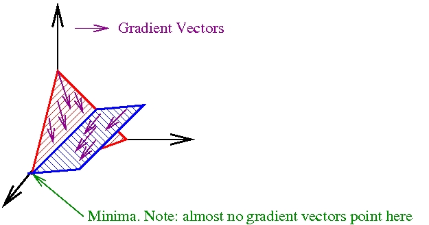
Gradient Descent	Specify an architecture with free parameters and use gradient descent with respect to data to tune the parameters.	Relatively computationally tractable due to (a) modularity of gradient descent (b) directly optimizing the quantity you want to predict.	Finicky. There are issues with paremeter initialization, step size, and representation. It helps a great deal to have accumulated experience using this sort of system and there is little theoretical guidance. Overfitting is a significant issue.
Kernel-based learning	You chose a kernel K(x,x’) between datapoints that satisfies certain conditions, and then use it as a measure of similarity when learning.	People often find the specification of a similarity function between objects a natural way to incorporate prior information for machine learning problems. Algorithms (like SVMs) for training are reasonably practical—O(n²) for instance.	Specification of the kernel is not easy for some applications (this is another example of prior elicitation). O(n²) is not efficient enough when there is much data.
Boosting	You create a learning algorithm that may be imperfect but which has some predictive edge, then apply it repeatedly in various ways to make a final predictor.	A focus on getting something that works quickly is natural. This approach is relatively automated and (hence) easy to apply for beginners.	The boosting framework tells you nothing about how to build that initial algorithm. The weak learning assumption becomes violated at some point in the iterative process.
Online Learning with Experts	You make many base predictors and then a master algorithm automatically switches between the use of these predictors so as to minimize regret.	This is an effective automated method to extract performance from a pool of predictors.	Computational intractability can be a problem. This approach lives and dies on the effectiveness of the experts, but it provides little or no guidance in their construction.
Learning Reductions	You solve complex machine learning problems by reducing them to well-studied base problems in a robust manner.	The reductions approach can yield highly automated learning algorithms.	The existence of an algorithm satisfying reduction guarantees is not sufficient to guarantee success. Reductions tell you little or nothing about the design of the base learning algorithm.
PAC Learning	You assume that samples are drawn IID from an unknown distribution D. You think of learning as finding a near-best hypothesis amongst a given set of hypotheses in a computationally tractable manner.	The focus on computation is pretty right-headed, because we are ultimately limited by what we can compute.	There are not many substantial positive results, particularly when D is noisy. Data isn’t IID in practice anyways.
Statistical Learning Theory	You assume that samples are drawn IID from an unknown distribution D. You think of learning as figuring out the number of samples required to distinguish a near-best hypothesis from a set of hypotheses.	There are substantially more positive results than for PAC Learning, and there are a few examples of practical algorithms directly motivated by this analysis.	The data is not IID. Ignorance of computational difficulties often results in difficulty of application. More importantly, the bounds are often loose (sometimes to the point of vacuousness).
Decision tree learning	Learning is a process of cutting up the input space and assigning predictions to pieces of the space.	Decision tree algorithms are well automated and can be quite fast.	There are learning problems which can not be solved by decision trees, but which are solvable. It’s common to find that other approaches give you a bit more performance. A theoretical grounding for many choices in these algorithms is lacking.
Algorithmic complexity	Learning is about finding a program which correctly predicts the outputs given the inputs.	Any reasonable problem is learnable with a number of samples related to the description length of the program.	The theory literally suggests solving halting problems to solve machine learning.
RL, MDP learning	Learning is about finding and acting according to a near optimal policy in an unknown Markov Decision Process.	We can learn and act with an amount of summed regret related to O(SA) where S is the number of states and A is the number of actions per state.	Has anyone counted the number of states in real world problems? We can’t afford to wait that long. Discretizing the states creates a POMDP (see below). In the real world, we often have to deal with a POMDP anyways.
RL, POMDP learning	Learning is about finding and acting according to a near optimaly policy in a Partially Observed Markov Decision Process	In a sense, we’ve made no assumptions, so algorithms have wide applicability.	All known algorithms scale badly with the number of hidden states.

This set is incomplete of course, but it forms a starting point for understanding what’s out there. (Please fill in the what/pro/con of anything I missed.)

11/27/2006

Continuizing Solutions

This post is about a general technique for problem solving which I’ve never seen taught (in full generality), but which I’ve found very useful.

Many problems in computer science turn out to be discretely difficult. The best known version of such problems are NP-hard problems, but I mean ‘discretely difficult’ in a much more general way, which I only know how to capture by examples.

ERM In empirical risk minimization, you choose a minimum error rate classifier from a set of classifiers. This is NP hard for common sets, but it can be much harder, depending on the set.
Experts In the online learning with experts setting, you try to predict well so as to compete with a set of (adversarial) experts. Here the alternating quantifiers of you and an adversary playing out a game can yield a dynamic programming problem that grows exponentially.
Policy Iteration The problem with policy iteration is that you learn a new policy with respect to an old policy, which implies that simply adopting the new policy can go very wrong.

For each of these problems, there are “continuized” solutions which can yield smaller computation, more elegant mathematics, or both.

ERM By shifting from choosing a single classifier to choosing a stochastic classifier we can prove a new style of bound which is significantly tighter, easier to state, and easier to understand than traditional bounds in the traditional setting. This is the PAC-Bayes bound idea.
Experts By giving the adversary slightly more power—the ability to split experts and have them fractionally predict one way vs. another, the optimal policy becomes much easier to compute (quadratic in the horizon, or maybe less). This is the continuous experts idea.
Policy Iteration For policy iteration, by stochastically mixing the old and the new policy, we can find a new policy better than the old policy. This is the conservative policy iteration idea.

There is some danger to continuizing. The first and second examples both involve a setting shift, which may not be valid—in general your setting should reflect your real problem rather than the thing which is easy to solve. However, even with the setting shift, the solutions appear so compellingly more elegant that it is hard to not hope to use them in a solution to the original setting.

I have not seen a good formulation of the general approach of continuizing. Nevertheless, I expect to see continuizing in more places and to use it in the future. By making it explicit, perhaps this can be made eaesier.