Gradients everywhere

One of the basic observations from the atomic learning workshop is that gradient-based optimization is pervasive. For example, at least 7 (of 12) speakers used the word ‘gradient’ in their talk and several others may be approximating a gradient. The essential useful quality of a gradient is that it decouples local updates from global optimization. Restated: Given a gradient, we can determine how to change individual parameters of the system so as to improve overall performance.

It’s easy to feel depressed about this and think “nothing has happened”, but that appears untrue. Many of the talks were about clever techniques for computing gradients where your calculus textbook breaks down.

  1. Sometimes there are clever approximations of the gradient. (Simon Osindero)
  2. Sometimes we can compute constrained gradients via iterated gradient/project steps. (Ben Taskar)
  3. Sometimes we can compute gradients anyways over mildly nondifferentiable functions. (Drew Bagnell)
  4. Even given a gradient, the choice of update is unclear, and might be cleverly chosen (Nic Schraudolph)

Perhaps a more extreme example of this is Adaboost which repeatedly reuses a classifier learner to implicitly optimize a gradient. Viewed as a gradient optimization algorithm, Adaboost is a sublinear algorithm (in the number of implicit parameters) when applied to decision trees.

The Approximation Argument

An argument is sometimes made that the Bayesian way is the “right” way to do machine learning. This is a serious argument which deserves a serious reply. The approximation argument is a serious reply for which I have not yet seen a reply2.

The idea for the Bayesian approach is quite simple, elegant, and general. Essentially, you first specify a prior P(D) over possible processes D producing the data, observe the data, then condition on the data according to Bayes law to construct a posterior:

P(D|x) = P(x|D)P(D)/P(x)

After this, hard decisions are made (such as “turn left” or “turn right”) by choosing the one which minimizes the expected (with respect to the posterior) loss.

This basic idea is reused thousands of times with various choices of P(D) and loss functions which is unsurprising given the many nice properties:

  1. There is an extremely strong associated guarantee: If the actual distribution generating the data is drawn from P(D) there is no better method. One way to think about this is that in the Bayesian setting, the worst case analysis is the average case analysis.
  2. The Bayesian method is a straightforward extension of the engineering method for designing a solution to a problem.
  3. The Bayesian method is modular. The three information sources are prior P(D), data x, and loss, but loss only interacts with P(D) and x via the posterior P(D|x).

The fly in the ointment is approximation. The basic claim of the approximation argument is that approximation is unavoidable in all real-world problems that we care about. There are several ways in which approximation necessarily invades applications of Bayes Law.

  1. When specifying the prior, the number of bits needed to describe the “real” P(D) is typically too large. The meaning of “real” P(D) actually varies, but this statement appears to hold true across all of them. What happens instead is that people take short-cuts specifying something which isn’t quite the real prior.
  2. Even if the real P(D) is somehow specifiable, computing the posterior P(D|x) is often computationally intractable. Again, the common short-cut is to alter the prior so as to make it computationally tractable. (There are a few people who instead attempt to approximately compute the posterior via monte carlo methods.)

Consider for example the problem of speech recognition. A “real” prior P(D) (according to some definitions) might involve a distribution over the placement of air molecules, the shape of the throat producing the sound, and what is being pronounced. This prior might be both inarticulable (prior elicitation is nontrivial) and unrepresentable (because too many bits are required to store on a modern machine).

If the necessity of approximation is accepted, the question becomes “what do you do about it?” There are many answers:

  1. Ignore the problem. This works well sometimes but can not be a universal prescription.
  2. Avoid approximation and work (or at least work a computer) very hard. This also can work well, at least for some problems.
  3. Use an approximate Bayesian method and leave a test set on the side to sanity check results. This is a common practical approach.
  4. Violate the modularity of loss and attempt to minimize approximation errors near the decision boundary. There seems to be little deep understanding of the viability and universality of this approach but there are examples where this approach can provide significant benefits.

Some non-Bayesian approaches can be thought of as attempts at (4).

Multitask learning is Black-Boxable

Multitask learning is the problem of jointly predicting multiple labels simultaneously with one system. A basic question is whether or not multitask learning can be decomposed into one (or more) single prediction problems. It seems the answer to this is “yes”, in a fairly straightforward manner.

The basic idea is that a controlled input feature is equivalent to an extra output. Suppose we have some process generating examples: (x,y1,y2) in S where y1 and y2 are labels for two different tasks. Then, we could reprocess the data to the form Sb(S) = {((x,i),yi): (x,y1,y2) in S, i in {1,2}} and then learn a classifier c:X x {1,2} -> Y. Note that (x,i) is the (composite) input. At testing time, given an input x, we can query c for the predicted values of y1 and y2 using (x,1) and (x,2).

A strong form of equivalence can be stated between these tasks. In particular, suppose we have a multitask learning algorithm ML which learns a multitask predictor m:X -> Y x Y. Then the following theorem can be proved:

For all ML for all S, there exists an inverse reduction Sm such that ML(S) = ML(Sm(Sb(S)).

In other words, no information is lost in the transformation Sb which means everything which was learnable previously remains learnable.

This may not be the final answer to the question because there may be some algorithm-dependent (mis)behavior associated with controlled feature i. It may also be the case that single task classification is computationally distinguishable from multitask classification. Certainly, computational concerns are one of the reasons specialized multitask classification algorithms exist.

Online learning or online preservation of learning?

In the online learning with experts setting, you observe a set of predictions, make a decision, and then observe the truth. This process repeats indefinitely. In this setting, it is possible to prove theorems of the sort:

master algorithm error count < = k* best predictor error count + c*log(number of predictors)

Is this a statement about learning or about preservation of learning? We did some experiments to analyze the new Binning algorithm which works in this setting. For several UCI datasets, we reprocessed them so that features could be used as predictors and then applied several master algorithms. The first graph confirms that Binning is indeed a better algorithm according to the tightness of the upper bound.


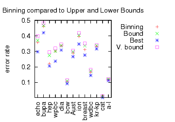
Here, “Best” is the performance of the best expert. “V. Bound” is the bound for Vovk‘s algorithm (the previous best). “Bound” is the bound for the Binning algorithm. “Binning” is the performance of the Binning algorithm. The Binning algorithm clearly has a tighter bound, and the performance bound is clearly a sharp constraint on the algorithm performance.

Instead of examining bounds, we can simply look at performance.


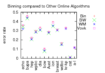
“Bin” is the performance of Binning (identical to the previous graph). BW is Binomial weighting, which is (roughly) the deterministic version of Binning. WM is Weighted Majority. Both BW and WM are deterministic algorithms which implies their performance bounds are perhaps a factor of 2 worse than Binning or Vovk’s algorithm.

In contrast, the actual performance (rather than performance bound) of the deterministic algorithms is sometimes even better than the best expert (negative regret?!). A consistent negative correlation between “online bound tightness” and “learning performance” is observed.

The question is “What’s happening here?”

  1. One reply is that we are testing in the wrong setting. These algorithms are designed to work in highly adversarial environments for which a UCI dataset does not qualify. This isn’t a convincing answer to me because many (or perhaps most) situations are not that adversarial.
  2. Another answer is “you used the wrong experts”. This is not convincing because many other learning algorithm do as well or better with the given features/experts.
  3. Another possibility is “you can start out running Binning, and when it pulls ahead of it’s bound run any learning algorithm. If the learning algorithm does badly, you can switch back to Binning and preserve the guarantee.” So, Binning is effectively a safety net.

My best current understanding is that “online learning with experts” is really “online preservation of learning”: the goal of the algorithm is to preserve whatever predictive ability the individual predictors have. This understanding fits the form of the theory statement well.

Preservation is desirable in some situations. For example, charity events sometimes work according to the following form:

  1. All participants exchange dollars for bogobucks.
  2. The participants gamble with bogobucks.
  3. The winner at the end gets some prize.

An online preservation algorithm has the property that if you acquire enough bogobucks in comparison to the number of participants, you can guarantee winning the prize. These kinds of ‘winner take all’ scenarios come up elsewhere.