HOMER: Provable Exploration in Reinforcement Learning

Last week at ICML 2020, Mikael Henaff, Akshay Krishnamurthy, John Langford and I had a paper on a new reinforcement learning (RL) algorithm that solves three key problems in RL: (i) global exploration, (ii) decoding latent dynamics, and (iii) optimizing a given reward function. Our ICML poster is here.

The paper is a bit mathematically heavy in nature so this post is an attempt to distill the key findings. We will also be following up soon with a new codebase release (more on it later).

Rich-observation RL landscape

Consider the combination lock problem shown below. The agent starts in the state s_1a or s_1b with equal probability. After taking h-1 actions, the agent will be in either state s_ha, s_hb, or s_hc. The agent can take 10 different actions. The agent observes a high-dimensional observation (focus circle) instead of the underlying state which is latent. There is a big treasure chest that one can get after taking 100 actions. We view the states with subscript “a” or “b” as “good states” and one with subscript “c” as “bad states”. You can reach the treasure chest at the end only if you remain in good states. If you reach any bad state, then you can never make it to the treasure chest.

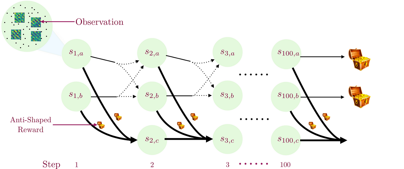
The environment makes it difficult to reach the big treasure chest in three ways. First, the environmental dynamics are such that if you are in good states, then only 1 out of 10 possible actions will let you reach the two good states at the next time step with equal probability (the good action changes from state to state). Every other action in good states and all actions in bad states put you into bad states at the next time step, from which it is impossible to recover. Second, it misleads myopic agents by giving a small bonus for transitioning from a good state to a bad state (small treasure chest). This means that a locally optimal policy is transitions to one of the bad states as quickly as possible. Third, the agent never directly observes which state it is in. Instead, it receives a high-dimensional, noisy observation from which it must decode the true underlying state.

It is easy to see that if we take actions uniformly at random, then the probability of reaching the big treasure chest at the end is 1/10¹⁰⁰. The number 10¹⁰⁰ is called Googol and is larger than the current estimate of number of elementary particles in the universe. Furthermore, since transitions are stochastic one can show that no fixed sequence of actions performs well either.

A key aspect of the rich-observation setting is that the agent receives observations instead of latent state. The observations are stochastically sampled from an infinitely large space conditioned on the state. However, observations are rich-enough to enable decoding the latent state which generates them.

What does provable RL mean?

A provable RL algorithm means that for any given numbers e, d in (0, 1); we can learn an e-optimal policy with probability at least 1-d using a number of episodes which are polynomial in relevant quantities (state size, horizon, action space, 1/e, 1/d, etc.). By e-optimal policy we mean a policy whose value (expected total return) is at most e less than the optimal return.

Thus, a provable RL algorithm is capable of learning a close to optimal policy with high probability (where the word high and close can be made arbitrarily more refined), provided the assumptions it makes are satisfied.

Why should I care if my algorithm is provable?

There are two main advantages of being able to show your algorithm is provable:

We can only test an algorithm on a finite number of environments (in practice somewhere between 1 and 20). Without guarantees, we don’t know how they will behave in a new environment. This matters especially if failure in a new environment can result in high real-world costs (e.g., in health or financial domains).
If a provable algorithm fails to consistently give the desired result, this can be attributed to failure of at least one of its assumptions. A developer can then look at the assumptions and try to determine which ones are violated, and either intervene to fix them or determine that the algorithm is not appropriate for the problem.

HOMER

Our algorithm addresses what is known as the Block MDP setting. In this setting, a small number of discrete states generates a potentially infinite number of high dimensional observations.

For each time step, HOMER learns a state decoder function, and a set of exploration policies. The state decoder maps high-dimensional observations to a small set of possible latent states, while the exploration policies map observations to actions which will lead the agent to each of the latent states. We describe HOMER below.

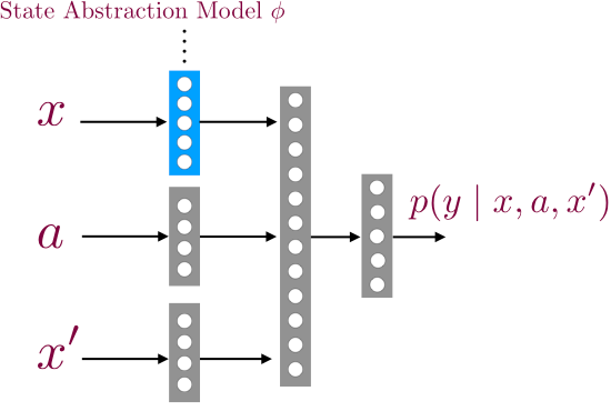
For a given time step, we first learn a decoder for mapping observations to a small set of values using contrastive learning. This procedure works as follows: collect a transition by following a randomly sampled exploration policy from the previous time step until that time step, and then taking a single random action. We use this procedure to sample two transitions shown below.

We then flip a coin; if we get heads then we store the transition (x1, a1, x’1), and otherwise we store the imposter transition (x1, a1, x’2). We train a supervised classifier to predict if a given transition (x, a, x’) is real or not.
This classifier has a special structure which allows us to recover a decoder for time step h.

Once we have learned the state decoder, we will learn an exploration policy for every possible value of the decoder (which we call abstract state as they are related to the latent state space). This step is standard can be done using many different approaches such as model-based planning, model-free methods, etc. In the paper we use an existing model-free algorithm called policy search by dynamic programming (PSDP) by Bagnell et al. 2004.

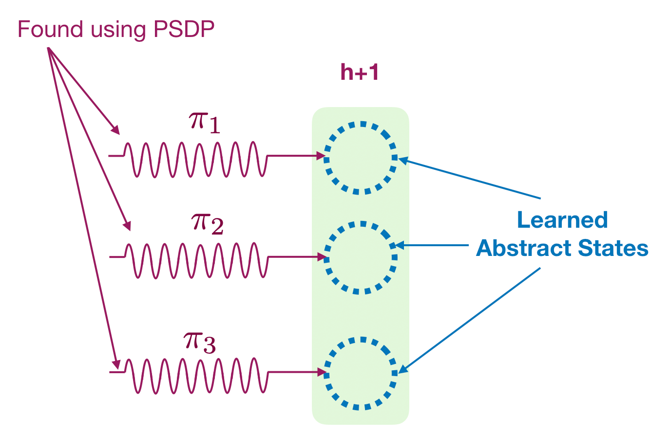
We recovered a decoder and a set of exploration policy for this time step. We then keep doing it for every time step and learn a decoder and exploration policy for the whole latent state space. Finally, we can easily optimize any given reward function using any provable planner like PSDP or a model-based algorithm. (The algorithm actually recovers the latent state space up to an inherent ambiguity by combining two different decoders; but I’ll leave that to avoid overloading this post).

Key findings

HOMER achieves the following three properties:

The contrastive learning procedure gives us the right state decoding (we recover up to some inherent ambiguity but I won’t cover it here).
HOMER can learn a set of exploration policies to reach every latent state
HOMER can learn a nearly-optimal policy for any given reward function with high probability. Further, this can be done after exploration part has been performed.

Failure cases of prior RL algorithms

There are many RL algorithms in the literature and many new are proposed every month. It is difficult to do justice to this vast literature in a blog post. It is equally difficult to situate HOMER in this vast literature. However, we show that several very commonly used RL algorithms fail to solve the above problem while HOMER succeeds. One of these is the PPO algorithm, a widely used policy gradient algorithm. In spite of its popular use, PPO is not designed for challenging exploration problems and easily fails. Researchers have made efforts to alleviate this with ad-hoc proposals such as using prediction errors, counts based on auto-encoders, etc. The best alternative approach we found is called Random Network Distillation(RND) which measures novelty of a state based on prediction errors for a fixed randomly initialized network.

Below we show how PPO+RND fails to solve the above problem while HOMER succeeds. We simplify the problem by using a grid pattern where rows represent the state (the top two represents “good” states and bottom row represents “bad” states), and column represents timestep.

We present counter-examples for other algorithms in the paper (see Section 6 here). These counterexamples allow us to find limits of prior work without expensive empirical computation on many domains.

How can I use with HOMER?

We will be providing the code soon as part of a new package release called cereb-rl. You can find it here: https://github.com/cereb-rl and join the discussion here: https://gitter.im/cereb-rl

6/7/2019

ICML has 3(!) Real World Reinforcement Learning Workshops

The first is Sunday afternon during the Industry Expo day. This one is meant to be quite practical, starting with an overview of Contextual Bandits and leading into how to apply the new Personalizer service, the first service in the world functionally supporting general contextual bandit learning.

The second is Friday morning. This one is more academic with many topics. I’ll personally be discussing research questions for real world RL.

The third one is Friday afternoon with more emphasis on sequences of decisions. I expect to here “imitation learning” multiple times 🙂

I’m planning to attend all 3. It’s great to see interest building in this direction, because Real World RL seems like the most promising direction for fruitfully expanding the scope of solvable machine learning problems.

7/6/2018

A Real World Reinforcement Learning Research Program

We are hiring for reinforcement learning related research at all levels and all MSR labs. If you are interested, apply, talk to me at COLT or ICML, or email me.

More generally though, I wanted to lay out a philosophy of research which differs from (and plausibly improves on) the current prevailing mode.

Deepmind and OpenAI have popularized an empirical approach where researchers modify algorithms and test them against simulated environments, including in self-play. They’ve achieved significant success in these simulated environments, greatly expanding the reportoire of ‘games solved by reinforcement learning’ which consisted of the singleton backgammon when I was a graduate student. Given the ambitious goals of these organizations, the more general plan seems to be “first solve games, then solve real problems”. There are some weaknesses to this approach, which I want to lay out next.

Broken API One issue with this is that multi-step reinforcement learning is a broken API in the sense that it creates an interface for problem definitions that is unsolvable via currently popular algorithm families. In particular, you can create problems which are either ‘antishaped’ so local rewards mislead w.r.t. long term rewards or keylock problems, as are common in Markov Decision Process lower bounds. I coded up simple versions of these problems a couple years ago and stuck them on github now to be extra crisp. If you try to apply policy gradient or Q-learning style algorithms on these problems they commonly run into exponential (in the number of states) sample complexity. As a general principle, APIs which create exponential sample complexity are bad—they imply that individual applications require taking advantage of special structure in order to succeed.
Transference Another significant issue is the degree of transference between solutions in simulation and the real world. “Transference” here potentially happens at several levels.
- Do the algorithms carry over? One of the persistent issues with simulation-based approaches is that you don’t care about sample complexity that much—optimal performance at acceptable computational complexities is the typical goal. In real world applications, this is somewhat absurd—you really care about immediately doing something reasonable and optimizing from there.
- Do the simulators carry over? For every simulator, there is a fidelity question which comes into play when you want to transfer a policy learned in the simulator into action in the real world. Real-time ray tracing and simulator quality more generally are advancing, but I’m not ready yet to trust a self-driving care trained in a simulated reality. An accurate simulation of the physics is unclear—friction for example is known-difficult, and more generally the representative variety of exogenous events in an open world seems quite difficult to implement.
Solution generality When you test and discover that an algorithm works in a simulated world, you know that it works in the simulated world. If you try it in 30 simulated worlds and it works in all of them, it can still easily be the case that an algorithm fails on the 31st simulated world. How can you achieve confidence beyond the number of simulated worlds that you try and succeed on? There is some sense by which you can imagine generalization over an underlying process generating problems, but this seems like a shaky justification in practice, since the nature of the problems encountered seems to be a nonstationary development of an unknown future.
Value creation Solutions of a ‘first A, then B’ flavor naturally take time to get to the end state where most of the real value is set to be realized. In the years before reaching applications in the real world, does the funding run out? We certainly hope not for the field of research but a danger does exist. Some discussion here including the comments is relevant.

What’s an alternative?

Each of the issues above is addressable.

Build fundamental theories of what are statistically and computationally tractable sub-problems of Reinforcement Learning. These tractable sub-problems form the ‘APIs’ of systems for solving these problems. Examples of this include simpler (Contextual Bandits), intermediate (learning to search, and move advanced (Contextual Decision Process).
Work on real-world problems. The obvious antidote to simulation is reality, driving both the need to create systems that work in reality as well as a research agenda around reality-centered issues like performance at low sample complexity. There are some significant difficulties with this—reinforcement style algorithms require interactive access to learn which often drives research towards companies with an infrastructure. Nevertheless, offline evaluation on real-world data does exist and the choice of emphasis in research directions is universal.
The combination of fundamental theories and a platform which distills learnings so they are not forgotten and always improved upon provides a stronger basis for expectation of generalization into the next problem.
The shortest path to creating valuable applications in the real world is to simply work on creating valuable applications in the real world. Doing this in a manner guided by other elements of the research program is just good sense.

The above must be applied in moderation—some emphasis on theory, some emphasis on real world applications, some emphasis on platforms, and some emphasis on empirics. This has been my research approach for a little over 10 years, ever since I started working on contextual bandits.

Let’s call the first research program ’empirical simulation’ and the second research program ‘real fundamentals’. The empirical simulation approach has a clear strong advantage in that it creates impressive demos, which creates funding, which creates more research. The threshold for contribution to the empirical simulation approach may also be lower simply because it requires mastery of fewer elements, implying people can more easily participate in it. At the same time, the real fundamentals approach has clear advantages in addressing the weaknesses of the empirical simulation approach. At a concrete level, this means we have managed to define and create fundamentals through research while creating real-world applications and value radically more efficiently than the empirical simulation approach has achieved.

The ‘real fundamentals’ concept is behind the open positions above. These positions have been designed to come with both the colleagues and mandate to address the most difficult research problems along with the organizational leverage to change the world. For people interested in fundamentals and making things happen in the real world these are prime positions—please consider joining us.

4/16/2018

Reinforcement Learning Platforms

If you are interested in building an industrial Reinforcement Learning platform, we are hiring a data scientist and multiple developers as a followup to last year’s hiring. Please apply if interested as this is a real chance to be a part of building the future 🙂

2/14/2018

Pervasive Simulator Misuse with Reinforcement Learning

The surge of interest in reinforcement learning is great fun, but I often see confused choices in applying RL algorithms to solve problems. There are two purposes for which you might use a world simulator in reinforcement learning:

Reinforcement Learning Research: You might be interested in creating reinforcement learning algorithms for the real world and use the simulator as a cheap alternative to actual real-world application.
Problem Solving: You want to find a good policy solving a problem for which you have a good simulator.

In the first instance I have no problem, but in the second instance, I’m seeing many head-scratcher choices.

A reinforcement learning algorithm engaging in policy improvement from a continuous stream of experience needs to solve an opportunity-cost problem. (The RL lingo for opportunity-cost is “advantage”.) Thinking about this in the context of a 2-person game, at a given state, with your existing rollout policy, is taking the first action leading to a win 1/2 the time good or bad? It could be good since the player is well behind and every other action is worse. Or it could be bad since the player is well ahead and every other action is better. Understanding one action’s long term value relative to another’s is the essence of the opportunity cost trade-off at the core of many reinforcement learning algorithms.

If you have a choice between an algorithm that estimates the opportunity cost and one which observes the opportunity cost, which works better? Using observed opportunity-cost is an almost pure winner because it cuts out the effect of estimation error. In the real world you can’t observe the opportunity cost directly Groundhog day style. How many times have you left a conversation and thought to yourself: I wish I had said something else? A simulator is different though—you can reset a simulator. And when you do reset a simulator, you can directly observe the opportunity-cost of an action which can then directly drive learning updates.

If you are coming from viewpoint 1, using a “reset cheat” is unappealing since it doesn’t work in the real world and the goal is making algorithms which work in the real world. On the other hand, if you are operating from viewpoint 2, the “reset cheat” is a gigantic opportunity to dramatically improve learning algorithms. So, why are many people with goal 2 using goal 1 designed algorithms? I don’t know, but here are some hypotheses.

Maybe people just aren’t aware that goal 2 style algorithms exist? They are out there. The most prominent examples of goal 2 style algorithms are from Learning to search and AlphaGo Zero.
Maybe people are worried about the additional sample complexity of doing multiple rollouts from reset points? But these algorithm typically require little additional sample complexity in the worst case and can provide gigantic wins. People commonly use a discount factor d values future rewards t timesteps ahead with a discount of d^t. Alternatively, you can terminate rollouts with probability 1 – d and value future rewards with no discount while preserving the expected value. Using this approach a rollout terminates after an expected 1/(1-d) timesteps bounding the cost of a reset and rollout. Since it is common to use very heavy discounting (e.g. d=0.9), the worst case additional sample complexity is only a small factor larger. On the upside, eliminating estimation error is can radically reduce sample complexity in theory and practice.
Maybe the implementation overhead for a second family of algorithms is to difficult? But the choice of whether or not you use resets is far more important than “oh, we’ll just run things for 10x longer”. It can easily make or break the outcome.

Maybe there is some other reason? As I said above, this is head-scratcher that I find myself trying to address regularly.