How is Compressed Sensing going to change Machine Learning ?

Compressed Sensing (CS) is a new framework developed by Emmanuel Candes, Terry Tao and David Donoho. To summarize, if you acquire a signal in some basis that is incoherent with the basis in which you know the signal to be sparse in, it is very likely you will be able to reconstruct the signal from these incoherent projections.

Terry Tao, the recent Fields medalist, does a very nice job at explaining the framework here. He goes further in the theory description in this post where he mentions the central issue of the Uniform Uncertainty Principle. It so happens that random projections are on average incoherent, within the UUP meaning, with most known basis (sines, polynomials, splines, wavelets, curvelets …) and are therefore an ideal basis for Compressed Sensing. [ For more in-depth information on the subject, the Rice group has done a very good job at providing a central library of papers relevant to the growing subject: http://www.dsp.ece.rice.edu/cs/ ]

The Machine Learning community has looked at Random Projections before, for instance:

  • Experiments with Random Projections for Machine Learning by Fradkin and Madigan (KDD-03.)
  • Face Recognition Experiments with Random Projection by Goel, Bebis and Nefian
  • Dimensionality reduction by random mapping: Fast similarity computation for clustering by S. Kaski (Proceedings of IEEE International Joint Conference on Neural Networks, 1998.)
  • but while they seem to give somewhat comparable results with regards to PCA, the number of contributions on the subject does not seem overwhelming. Maybe one of the reason is that in most papers cited above, the main theoretical reason for using Random projections lies with the Johnson-Lindenstrauss (JL) lemma. As a consequence, most random matrices used in these publications come from the Database world and not from the newer framework of Compressed Sensing (a list of these matrices and their properties can be found in the middle of this page). The uncanny reliance on Random projections within the JL lemma and in the Compressed Sensing setting was explained by Richard Baraniuk, Mark Davenport, Ronald DeVore, and Michael Wakin in this paper entitled: A simple proof of the restricted isometry property for random matrices. However, the most interesting fallout from this comparison between JL and CS comes in the form of the contribution by Richard Baraniuk and Michael Wakin in Random projections of smooth manifolds. I’ll let the abstract speak for itself:

    We propose a new approach for nonadaptive dimensionality reduction of manifold-modeled data, demonstrating that a small number of random linear projections can preserve key information about a manifold-modeled signal……As our main theoretical contribution, we establish a sufficient number M of random projections to guarantee that, with high probability, all pairwise Euclidean and geodesic distances between points on M are well-preserved under the mapping \phi. Our results bear strong resemblance to the emerging theory of Compressed Sensing (CS), in which sparse signals can be recovered from small numbers of random linear measurements. As in CS, the random measurements we propose can be used to recover the original data in RN. Moreover, like the fundamental bound in CS, our requisite M is linear in the “information level” K and logarithmic in the ambient dimension N; we also identify a logarithmic dependence on the volume and curvature of the manifold. In addition to recovering faithful approximations to manifold-modeled signals, however, the random projections we propose can also be used to discern key properties about the manifold. We discuss connections and contrasts with existing techniques in manifold learning, a setting where dimensionality reducing mappings are typically nonlinear and constructed adaptively from a set of sampled training data.

    It looks as though, as a result, Universal Dimensionality Reduction is achieved by some properly chosen random projections. In the case of data living in a low dimensional manifold, the JL lemma states that the number of random projections is proportional to the number of points or samples from that manifold, on the other hand, CS seems to show that the number of random projections is proportional to the characteristic of the manifold only.

    The results highlighted by Wakin and Baraniuk are very compelling but there is another appealing reason to Random Projections: Robustness. While trying to mimick nature in the learning process, one cannot but be amazed at the reliability of the biological system. On the other hand, even the researchers that model these processes do not realize or point out that this robustness is in part due to random projections. Case in point, the excellent work of Thomas Serre, Aude Oliva and Tomaso Poggio culminating in a paper describing a biology inspired model of brain that shows its ability to process information in a feedforward fashion. The modeling is new in that, in this area of science, there is a central issue as to whether the brain works in a one-way process or with many loops. In the paper, the feature dimension reduction model (which is what this process is) uses random projections as I pointed out recently.

    Because of the intrinsic dimension reduction capability, Mike Wakin has also shown efficient nearest neighbor searches using few random projections (see figure 3 of this paper). I could go on but the point is that since CS is a revolution in the world of signal/feature acquisition and processing (see the analog-to-information A2I site ) one cannot but wonder aloud how this will affect Machine Learning in general.
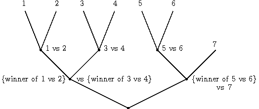
    Conditional Tournaments for Multiclass to Binary

    This problem has been cracked (but not quite completely solved) by Alina, Pradeep, and I. The problem is essentially finding a better way to reduce multiclass classification to binary classification. The solution is to use a carefully crafted tournament, the simplest version of which is a single elimination tournament where the “players” are the different classes. An example of the structure is here:


    For the single elimination tournament, we can prove that:
    For all multiclass problems D, for all learned binary classifiers c, the regret of an induced multiclass classifier is bounded by the regret of the binary classifier times log2 k. Restated:

    regmulticlass(D,Filter_tree_test(c)) <= regbinary (Filter_tree_train(D),c)

    Here:

    1. Filter_tree_train(D) is the induced binary classification problem
    2. Filter_tree_test(c) is the induced multiclass classifier.
    3. regmulticlass is the multiclass regret (= difference between error rate and minimum possible error rate)
    4. regbinary is the binary regret

    This result has a slight dependence on k which we suspect is removable. The current conjecture is that this dependence can be removed by using higher order tournaments such as double elimination, triple elimination, up to log2 k-elimination.

    The key insight which makes the result possible is conditionally defining the prediction problems at interior nodes. In essence, we use the learned classifiers from the first level of the tree to filter the distribution over examples reaching the second level of the tree. This process repeats, until the root node is reached. Further details, including a more precise description and some experimental results are in the draft paper.

    Alternative Machine Learning Reductions Definitions

    A type of prediction problem is specified by the type of samples produced by a data source (Example: X x {0,1}, X x [0,1], X x {1,2,3,4,5}, etc…) and a loss function (0/1 loss, squared error loss, cost sensitive losses, etc…). For simplicity, we’ll assume that all losses have a minimum of zero.

    For this post, we can think of a learning reduction as

    1. A mapping R from samples of one type T (like multiclass classification) to another type T’ (like binary classification).
    2. A mapping Q from predictors for type T’ to predictors for type T.

    The simplest sort of learning reduction is a “loss reduction”. The idea in a loss reduction is to prove a statement of the form:
    Theorem For all base predictors b, for all distributions D over examples of type T:

    E(x,y) ~ D LT(y,Q(b,x)) <= f(E(x’,y’)~R(D) LT’(y’,b(x’)))

    Here LT is the loss for the type T problem and LT’ is the loss for the type T’ problem. Also, R(D) is the distribution over samples induced by first drawing from D and then mapping the sample via R. The function f() is the loss transform function—we try to find reductions R,Q which minimize it’s value.

    If R,Q are deterministic, then there always exists a choice of D,b such that the loss rate on the right hand side is 0. However, it’s common to encounter real-world learning problems D which are inherently noisy, implying that the induced problem D’ is often inherently noisy. Distinguishing between errors due to environmental noise and errors due to base predictor mistakes seems important (and experimentally, it has been). Regret transform reductions can get at this. They have theorems of the form:
    Theorem For all base predictors b, for all distributions D over examples of type T:

    E(x,y) ~ D LT(y,Q(b,x)) – minc E(x,y) ~ D LT(y,c(x)) <= f(E(x’,y’)~R(D) LT’(y’,b(x’)) – minb’ E(x’,y’)~R(D) LT’(y’,b'(x’)))

    The essential idea in regret transform reductions is that we subtract off the inherent noise in both the induced and original problem, and bound the excess loss due to suboptimal prediction directly.

    The skeletons of the theory for these families of reductions have been layed out at this point. There remain some open problems, but another interesting direction to consider is other families of reductions. The hope is that by placing more stringent requirements on reductions, we limit ourselves to algorithms which tend to perform better in practice. This hope is pretty reasonable—empirically, we have observed a consistent step up in performance going from loss transform to regret transform reductions.

    1. Limited Regret Transform Reductions. The fact that the minimum is taken over all predictors in regret transforms is counterintuitive to some people, who are used to “Empirical Risk Minimization” statements where a minimum is taken over a limited set of predictors. We could imagine theorem statements of the form:
      Theorem For all sets of base predictors B, For all base predictors b, for all distributions D over examples of type T:
      E(x,y) ~ D LT(y,Q(b,x)) – minb’ in B E(x,y) ~ D LT(y,Q(b’,x)) <= f(E(x’,y’)~R(D) LT’(y’,b(x’)) – minb’ in B E(x’,y’)~R(D) LT’(y’,b'(x’)))

      This is a more general statement than a regret transform reduction—when B is the set of all base predictors, we recover standard regret transforms
      One case where it’s easy to see that this kind of statement holds is for the reduction from importance weighted binary classification to binary classification. However, little more is currently known.
    2. Reversible Reductions. This is an idea which Russell Impagliazzo first mentioned to me. Essentially, we limit ourselves to reductions with the property that they are reversible. Reversibility can be tested by mapping from one problem to another, and then back. There are a several variant theorem statements we could imagine. The most tractable variant for analysis might be the following:
      Theorem There exists R-1,Q-1 such that for all base predictors b, for base learning problems D’:
      E(x’,y’)~D’ LT’(y’,b(x’)) = E(x’,y’) ~ R(R-1(D’)) LT’(y’,b(x’))

      and Q-1(Q(b))=b

      Closely related (but different) is the following:
      Theorem There exists R-1,Q-1 such that for all type T predictors h, for all type T distributions D:
      E(x,y) ~ D LT(y,h(x)) = E(x,y)~R-1(R(D)) LT(y,h(x))

      and Q(Q-1(h)) = h
    3. Bayesian Reductions This is an idea which Simon Osindero mentioned. The basic observation is that Bayes Law is pretty important to the process of learning. We would like it to be the case that Bayes Law and reductions compose. A theorem statement of the following form might be about right.
      Theorem For some large family of priors P over distributions D of type T:
      Bayes(P,(x,y)~D~P) = Q(Bayes(R(P),(x’,y’)~D’~R(P)))

      Here “Bayes” is a learning algorithm which takes as input a prior P (or R(P)), and a sample (x,y) drawn by first drawing a D from P and then drawing from D (and similarly for the induced problem). Also, R(P) is the prior induced by mapping D to R(D) after drawing from P.

    The two missing components for these kinds of reductions are:

    1. Theoretical evidence that we can satisfy these definitions of reduction between interesting types of learning problems.
    2. Empirical evidence that algorithmic modifications driven by the theory are useful.

    My experience is that analyzing reductions has yielded significant insight into how to solve learning problems, so I would encourage anyone with a bit of theoretical inclination in Machine Learning to consider the above (or other) families of reductions.

    All Models of Learning have Flaws

    Attempts to abstract and study machine learning are within some given framework or mathematical model. It turns out that all of these models are significantly flawed for the purpose of studying machine learning. I’ve created a table (below) outlining the major flaws in some common models of machine learning.

    The point here is not simply “woe unto us”. There are several implications which seem important.

    1. The multitude of models is a point of continuing confusion. It is common for people to learn about machine learning within one framework which often becomes there “home framework” through which they attempt to filter all machine learning. (Have you met people who can only think in terms of kernels? Only via Bayes Law? Only via PAC Learning?) Explicitly understanding the existence of these other frameworks can help resolve the confusion. This is particularly important when reviewing and particularly important for students.
    2. Algorithms which conform to multiple approaches can have substantial value. “I don’t really understand it yet, because I only understand it one way”. Reinterpretation alone is not the goal—we want algorithmic guidance.
    3. We need to remain constantly open to new mathematical models of machine learning. It’s common to forget the flaws of the model that you are most familiar with in evaluating other models while the flaws of new models get exaggerated. The best way to avoid this is simply education.
    4. The value of theory alone is more limited than many theoreticians may be aware. Theories need to be tested to see if they correctly predict the underlying phenomena.

    Here is a summary what is wrong with various frameworks for learning. To avoid being entirely negative, I added a column about what’s right as well.

    Name Methodology What’s right What’s wrong
    Bayesian Learning You specify a prior probability distribution over data-makers, P(datamaker) then use Bayes law to find a posterior P(datamaker|x). True Bayesians integrate over the posterior to make predictions while many simply use the world with largest posterior directly. Handles the small data limit. Very flexible. Interpolates to engineering.
    1. Information theoretically problematic. Explicitly specifying a reasonable prior is often hard.
    2. Computationally difficult problems are commonly encountered.
    3. Human intensive. Partly due to the difficulties above and partly because “first specify a prior” is built into framework this approach is not very automatable.
    Graphical/generative Models Sometimes Bayesian and sometimes not. Data-makers are typically assumed to be IID samples of fixed or varying length data. Data-makers are represented graphically with conditional independencies encoded in the graph. For some graphs, fast algorithms for making (or approximately making) predictions exist. Relative to pure Bayesian systems, this approach is sometimes computationally tractable. More importantly, the graph language is natural, which aids prior elicitation.
    1. Often (still) fails to fix problems with the Bayesian approach.
    2. In real world applications, true conditional independence is rare, and results degrade rapidly with systematic misspecification of conditional independence.
    Convex Loss Optimization Specify a loss function related to the world-imposed loss fucntion which is convex on some parametric predictive system. Optimize the parametric predictive system to find the global optima. Mathematically clean solutions where computational tractability is partly taken into account. Relatively automatable.
    1. The temptation to forget that the world imposes nonconvex loss functions is sometimes overwhelming, and the mismatch is always dangerous.
    2. Limited models. Although switching to a convex loss means that some optimizations become convex, optimization on representations which aren’t single layer linear combinations is often difficult.
    Gradient Descent Specify an architecture with free parameters and use gradient descent with respect to data to tune the parameters. Relatively computationally tractable due to (a) modularity of gradient descent (b) directly optimizing the quantity you want to predict.
    1. Finicky. There are issues with paremeter initialization, step size, and representation. It helps a great deal to have accumulated experience using this sort of system and there is little theoretical guidance.
    2. Overfitting is a significant issue.
    Kernel-based learning You chose a kernel K(x,x’) between datapoints that satisfies certain conditions, and then use it as a measure of similarity when learning. People often find the specification of a similarity function between objects a natural way to incorporate prior information for machine learning problems. Algorithms (like SVMs) for training are reasonably practical—O(n2) for instance. Specification of the kernel is not easy for some applications (this is another example of prior elicitation). O(n2) is not efficient enough when there is much data.
    Boosting You create a learning algorithm that may be imperfect but which has some predictive edge, then apply it repeatedly in various ways to make a final predictor. A focus on getting something that works quickly is natural. This approach is relatively automated and (hence) easy to apply for beginners. The boosting framework tells you nothing about how to build that initial algorithm. The weak learning assumption becomes violated at some point in the iterative process.
    Online Learning with Experts You make many base predictors and then a master algorithm automatically switches between the use of these predictors so as to minimize regret. This is an effective automated method to extract performance from a pool of predictors. Computational intractability can be a problem. This approach lives and dies on the effectiveness of the experts, but it provides little or no guidance in their construction.
    Learning Reductions You solve complex machine learning problems by reducing them to well-studied base problems in a robust manner. The reductions approach can yield highly automated learning algorithms. The existence of an algorithm satisfying reduction guarantees is not sufficient to guarantee success. Reductions tell you little or nothing about the design of the base learning algorithm.
    PAC Learning You assume that samples are drawn IID from an unknown distribution D. You think of learning as finding a near-best hypothesis amongst a given set of hypotheses in a computationally tractable manner. The focus on computation is pretty right-headed, because we are ultimately limited by what we can compute. There are not many substantial positive results, particularly when D is noisy. Data isn’t IID in practice anyways.
    Statistical Learning Theory You assume that samples are drawn IID from an unknown distribution D. You think of learning as figuring out the number of samples required to distinguish a near-best hypothesis from a set of hypotheses. There are substantially more positive results than for PAC Learning, and there are a few examples of practical algorithms directly motivated by this analysis. The data is not IID. Ignorance of computational difficulties often results in difficulty of application. More importantly, the bounds are often loose (sometimes to the point of vacuousness).
    Decision tree learning Learning is a process of cutting up the input space and assigning predictions to pieces of the space. Decision tree algorithms are well automated and can be quite fast. There are learning problems which can not be solved by decision trees, but which are solvable. It’s common to find that other approaches give you a bit more performance. A theoretical grounding for many choices in these algorithms is lacking.
    Algorithmic complexity Learning is about finding a program which correctly predicts the outputs given the inputs. Any reasonable problem is learnable with a number of samples related to the description length of the program. The theory literally suggests solving halting problems to solve machine learning.
    RL, MDP learning Learning is about finding and acting according to a near optimal policy in an unknown Markov Decision Process. We can learn and act with an amount of summed regret related to O(SA) where S is the number of states and A is the number of actions per state. Has anyone counted the number of states in real world problems? We can’t afford to wait that long. Discretizing the states creates a POMDP (see below). In the real world, we often have to deal with a POMDP anyways.
    RL, POMDP learning Learning is about finding and acting according to a near optimaly policy in a Partially Observed Markov Decision Process In a sense, we’ve made no assumptions, so algorithms have wide applicability. All known algorithms scale badly with the number of hidden states.

    This set is incomplete of course, but it forms a starting point for understanding what’s out there. (Please fill in the what/pro/con of anything I missed.)

    Incompatibilities between classical confidence intervals and learning.

    Classical confidence intervals satisfy a theorem of the form: For some data sources D,

    PrS ~ D(f(D) > g(S)) > 1-d

    where f is some function of the distribution (such as the mean) and g is some function of the observed sample S. The constraints on D can vary between “Independent and identically distributed (IID) samples from a gaussian with an unknown mean” to “IID samples from an arbitrary distribution D“. There are even some confidence intervals which do not require IID samples.

    Classical confidence intervals often confuse people. They do not say “with high probability, for my observed sample, the bounds holds”. Instead, they tell you that if you reason according to the confidence interval in the future (and the constraints on D are satisfied), then you are not often wrong. Restated, they tell you something about what a safe procedure is in a stochastic world where d is the safety parameter.

    There are a number of results in theoretical machine learning which use confidence intervals. For example,

    1. The E3 algorithm uses confidence intervals to learn a near optimal policy for any MDP with high probability.
    2. Set Covering Machines minimize a confidence interval upper bound on the true error rate of a learned classifier.
    3. The A2 uses confidence intervals to safely deal with arbitrary noise while taking advantage of active learning.

    Suppose that we want to generalize thse algorithms in a reductive style. The goal would be to train a regressor to predict the output of g(S) for new situations. For example, a good regression prediction of g(S) might allow E3 to be applied to much larger state spaces. Unfortunately, this approach seems to fail badly due to a mismatch between the semantics of learning and the semantics of a classical confidence interval.

    1. It’s difficult to imagine a constructive sampling mechanism. In a large state space, we may never encounter the same state twice, so we can not form meaningful examples of the form “for this state-action, the correct confidence interval is y“.
    2. When we think of succesful learning, we typically think of it in an l1 sense—the expected error rate over the data generating distribution is small. Confidence intervals have a much stronger meaning as we would like to apply them: with high probability, in all applications, the confidence interval holds. This mismatch appears unaddressable.

    It is tempting to start plugging in other notions such as Bayesian confidence intervals or quantile regression systems. Making these approaches work at a theoretical level on even simple systems is an open problem, but there is plenty of motivation to do so.